⛅ Seeing Through Clouds
During the 2020 lockdown, I embarked on building machine learning applications using satellite images with the lovely folks from ruumi.io. We worked on machine learning models to look through clouds, in collaboration with daniel-j-h.
We recently presented our approach on cloud see-thru at the GeoBerlin meetup, and received a lot of interest and questions. And so, we decided to write this blog post detailing our methodology, and challenges we faced on the way.
The Challenges with using Satellite Images⌗
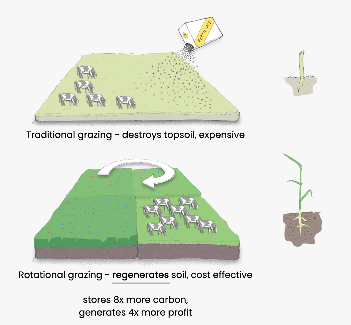
At ruumi, we work on rotational grazing: a managed grazing technique to improve biodiversity, replenish the soil, and be profitable for farmers at the same time. However, many farmers are apprehensive about adopting such regenerative agriculture techniques, as they are labor-intensive and require complex planning.
This is where ruumi comes in: we are using multi-spectral and radar satellite images, soil maps, seed mix data, and state-of-the-art remote sensing and machine learning techniques to assist farmers in transitioning to regenerative agriculture.
One of the main challenges in using satellite data for land monitoring applications is cloud obstruction. These obstructions can be twofold: clouds may block the view of the farmland underneath and their shadows may obscure or distort features on the ground.
Over the last few years, several cloud removal techniques have been developed: Sentinel-2 Cloudless, Mapbox Cloudless Atlas and Google’s Cloudless Satellite Map. These techniques are sifting through multiple years of images to create cloud-free scenes. This works fine if the goal is to improve the aesthetics of the satellite images, but the trade-off is recency. In applications like ours, where we rely on the most recent images to monitor changes on the land, these techniques cannot be used.
Since we haven’t found any cloud removal techniques out there that prioritize recency, we set out to develop our own state-of-the-art machine learning model to do just that. Our goal is not to hallucinate what we can’t see, but instead, to remove those pesky translucent clouds and accurately reconstruct what’s underneath.
 Before and after pictures showing our cloud removal technique
Sentinel-2 Constellation⌗
Over the past decade, the European Space Agency (ESA) has been developing and putting into orbit, a network of satellites called Sentinels. These satellites carry a range of sensors, such as radar and multi-spectral imaging instruments for land, ocean, and atmospheric monitoring at a global scale.
The Sentinel-2 satellite mission is part of this ongoing effort and is of particular interest to us. This mission consists of twin satellites flying in the same orbit around the earth, but phased at 180°. They provide high resolution multi-spectral images with a planet wide coverage, and a revisit frequency of 3-5 days i.e. the satellite sensors revisit the same patch on the earth every 3-5 days.
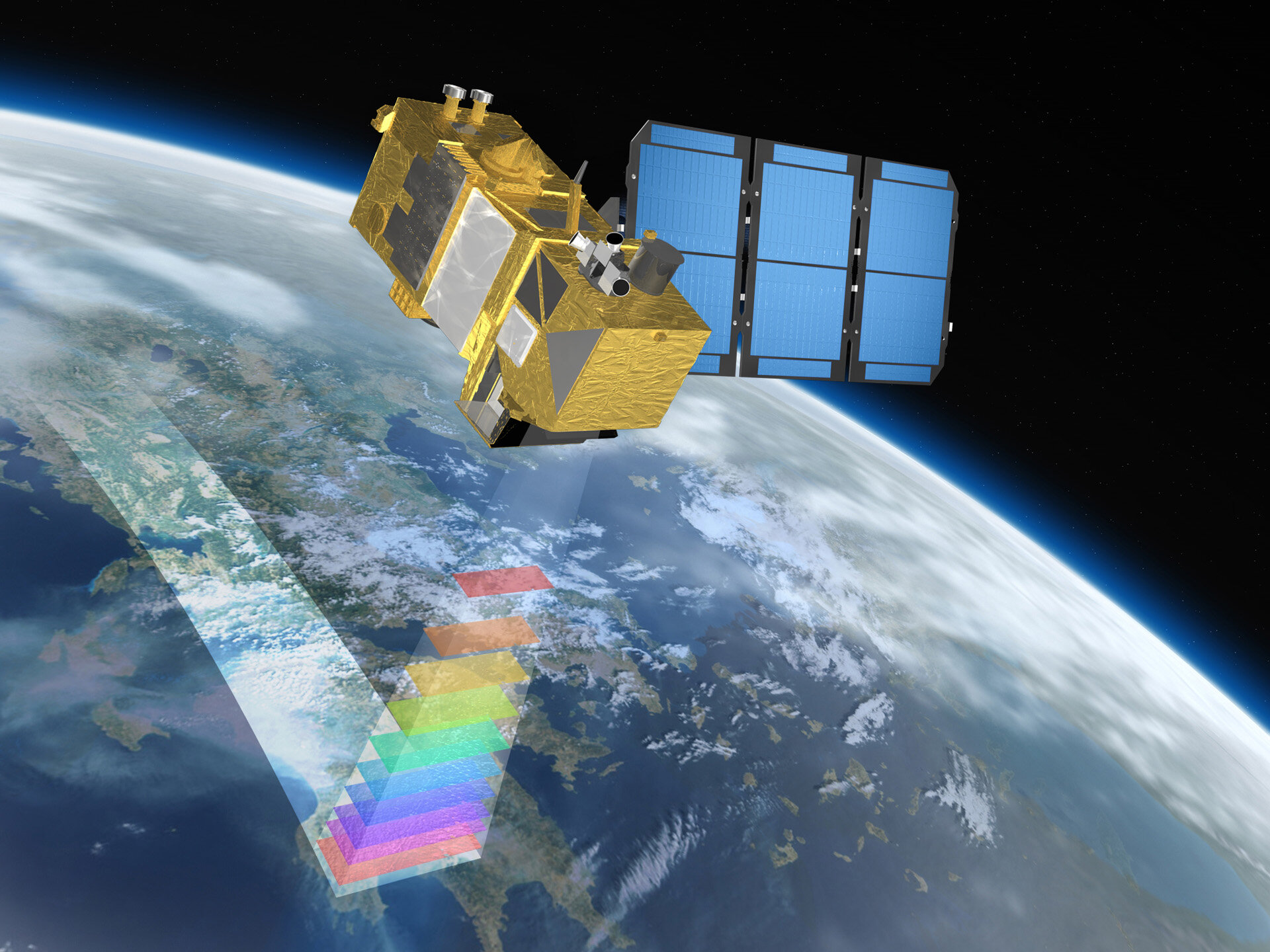 Sentinel 2 satellite, mapping the earth’s surface. Photo by ESA
The Sentinel-2 satellites carry a multi-spectral instrument (MSI) which works passively, by collecting sunlight reflected from the Earth’s surface. New data is acquired as the satellite moves along its orbital path. The incoming light beam is split into 12 spectral bands, in the visible, near infrared and short wave infrared spectral range. Of these 12 bands, 4 bands are at 10m, 6 bands at 20m and 2 bands at 60m spatial resolution. Here, spatial resolution refers to the ground area covered by one pixel. This means that in an image of 10m resolution, each pixel corresponds to a square of 10m x 10m on the ground.
Apart from these 12 spectral bands, Sentinel-2 data also includes a scene classification mask at 60m resolution. With the help of this band we can easily identify defective pixels, cloud pixels (both thick and thin or cirrus), snow or water pixels, and vegetation and non-vegetation pixels in the image.
For more information on the Sentinel-2 mission, please refer to their user guides.
Cloud Mask⌗
Clouds can be broadly classified into two types: dense, and thin or cirrus clouds.
Dense clouds do not allow the penetration of visible spectral radiation from the ground and tend to cast a shadow on the ground. It is hard to predict the pixel values under these clouds with high confidence as none of the Sentinel-2 spectral bands are able to penetrate through them.
Thin or cirrus clouds on the other hand are transparent or semi-transparent clouds. Most spectral bands can partially see through these clouds. This is key to accurate de-clouding with our model.
The scene classification mask provided in Sentinel-2 data is able to classify cloud pixels and cloud shadows in the image. It is also able to distinguish between thick and cirrus clouds, as described here.
Our aim is to reconstruct pixels classified as cirrus clouds and cloud shadows, while guaranteeing image recency and accuracy.
Our Approach⌗
Our main contribution is to create a training dataset based on (cloud, no-cloud) pairs for the same geography but from different days. The machine learning model then learns to re-construct the no-cloud sample from the cloud sample.
The basic assumption is that between cloud and no-cloud scenes only cloud pixels will change. This simple approach worked very well for us.
Inspired by the paper Image inpainting for irregular holes using partial convolutions, we developed a machine learning model that can reconstruct pixels that are otherwise distorted by the semi-transparent clouds and cloud shadows. We pass image data from the 12 multi-spectral bands, and the cloud mask extracted from the scene classification mask to our model. Our model, referred to as SensrUnet, works by extracting relevant information from the multi-spectral image data and reconstructing a de-clouded image from the information.
To prepare our training dataset, we began by downloading Sentinel-2 tiles from the past two years over the geographical region of Germany. There are multiple Sentinel-2 tiles covering Germany and we use all tiles to build a dataset to train our model.
 Sentinel tile cover over Germany
The spatial resolutions of the multi-spectral bands varied between 10m, 20m and 60m resolution. To stack all the bands together, so that it can be passed to the model as a single input unit, bands have to be scaled to the same resolution. Scaling bands from lower resolution to a higher resolution, inadvertently results in introducing blurriness. To keep this to a minimum and since most of the bands were in the 20m and 60m spatial resolution, we chose to scale all the bands to 20m resolution.
 Cutting out smaller images from the spectral band stacks
We stacked all the 12 resampled spectral bands, and the cloud mask generated from the scene classification mask. Next we cut out smaller images of size 256x256x13 from these spectral band stacks and constructed (cloud, no-cloud) image pairs.
To assure recency between the cloud and no-cloud images, we constrained the time difference between these images to be at most two weeks.
Network Architecture⌗
SensrUNet is an improved UNet architecture with a pre-trained encoder following the approach from the TernausNet paper. The decoder blocks perform pixel shuffle up-scaling with ICNR initialization to avoid any artifacts in the up-scaled image.
We also added global context attention blocks after each encoder and decoder layer. These attention blocks enable the model to reconstruct different parts of the image effectively as they retain a global context of the image. We observed significant improvements in output image quality with the attention blocks, while the number of parameters increased only by a small percentage of 1.6%.
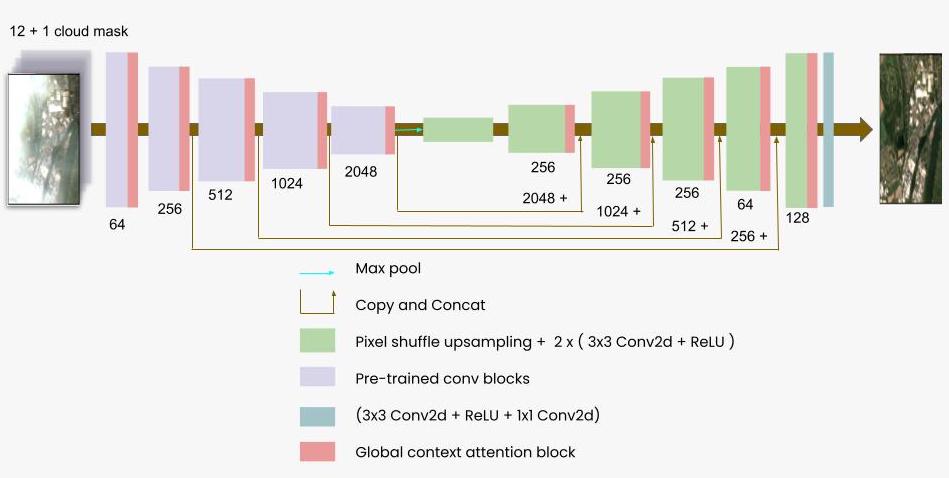 SensrUnet: model architecture
Loss Function and Model⌗
Our training dataset consists of (cloud, no-cloud) pairs. We pass the cloudy image (with 13 multi-spectral bands) to our model, and it outputs a de-clouded image, which we compare to the no-cloud image (target image).
Since we don’t want the model to strongly replicate the pixel values in the target image, we focus on loss computation only on pixels where thin or cirrus clouds are present. We uniquely designed our loss function to be a combination of pixel loss, perceptual, texture losses and total variation loss, similar to the loss function used in this paper.
The perceptual and texture losses allow for minor fluctuations between the output and target, while capturing the similarity in style and the features of the two images. After all, these are satellite images of two different days and minor variations in the input and target images are expected.
The total variation loss, acts as a smoothing penalty on the composite image. Collectively, these loss functions ensure smooth reconstruction of the image under thin or cirrus cloud pixels.
composite = cloud_mask * out + (1 - cloud_mask) * target

loss = a * PixelwiseLoss(cloud_mask * out, cloud_mask * target)
     + b * PerceptualLoss(composite, target)
     + c * TextureLoss(composite, target)
     + d * VariationLoss(composite)
Weighted combination of individual loss-terms
We trained the model for 48 hours on our workstation with 2x NVIDIA RTX 2080 TIs.
During inference, we ensure that we modify only pixels where thin or cirrus clouds are present and copy the other pixel values as is from the input image. The reason for this is, that we don’t want to introduce prediction uncertainty in pixels where there were no clouds present, and leave those pixels untouched.
Before and after pictures showing our cloud removal technique
Future Work⌗
We set out to develop a state-of-the art machine learning model that can de-cloud satellite images while prioritizing image recency. Using SensrUnet, and the scene classification mask, we are able to successfully see through thin or cirrus clouds.
However, we found that the scene classification mask provided by Sentinel-2 is often unreliable. We came across instances where dense clouds pixels were incorrectly classified as see-through clouds. When predicting on such pixels, the model inaccurately hallucinates the underlying pixel values which lead to random outputs in these pixels. We also found thin cloud pixels incorrectly classified as dense clouds, and so we aren’t able to remove all thin cloud pixels in the predicted image.
It might be worth looking into learning de-clouding and cloud segmentation simultaneously: learning the de-clouded bands, and learning a cloud mask that represents thin clouds at the same time. The learned cloud mask would then represent clouds we can and can not see through with multi-spectral bands.
We can also benefit from incorporating Sentinel-1’s SAR (satellite radar) to the training dataset, which is easily possible. The radar data can peek through both thin and thick clouds, unlike Sentinel-2’s sensors.
About The Author⌗
Sowmya is an independent contributor at ruumi, developing state-of-the-art machine learning techniques for satellite images.
Want to leave feedback? Reach out at hello@ruumi.io